Trigonometrie
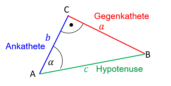
Winkelberechnung am Dreieck
Trigonometrie am Einheitskreis
Visualisierung von sin(α) und cos(α)
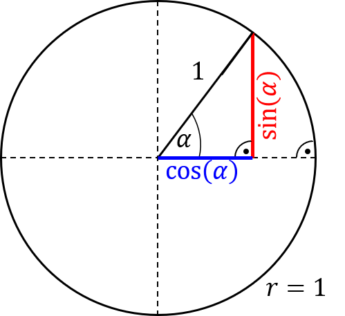
Im Einheitskreis lässt sich für beliebige Winkel α jeweils ein rechtwinkliges Dreieck konstruieren,
wie es auf der Abbildung oben gezeigt ist.
Die Hypotenuse in diesem rechtwinkligen Dreieck hat die Länge 1.
Nach Definition gilt:
sin(α)=HypotenuseGegenkathete,cos(α)=HypotenuseAnkathete
Folglich entspricht die Länge der Gegenkathete im dargestellten Dreieck direkt sin(α). Analog dazu lässt sich über die Länge der Ankathete der cos(α) bestimmen.
Nach dem Satz des Pythagoras gilt:
sin2(α)+cos2(α)=1
Variieren Sie in der folgenden Abbildung über den Schieberegler den Winkel α und beobachten Sie, wie sich das Dreieck und damit verbunden die Werte für sin(α) und cos(α) ändern.
Auf der rechten Seite sehen Sie als Ergänzung die Funktionsschaubilder der Funktionen sin(α) (schwarze Linie) und cos(α) (grau gestrichelte Linie).
Dort lassen sich ebenfalls die Funktionswerte für den eingestellten Winkel α ablesen.
import numpy as np
from bokeh.plotting import figure, show
from bokeh.models import Slider, ColumnDataSource, CustomJS, Label
from bokeh.layouts import column, row
from bokeh.io import output_notebook

output_notebook()

theta = np.linspace(0, 2*np.pi, 100)
deg = theta / np.pi * 180
x_circle = np.cos(theta)
y_circle = np.sin(theta)
sin_curve = np.sin(theta)
cos_curve = np.cos(theta)
alpha_init = 30
phi_init = np.deg2rad(alpha_init)

# Datenquellen
source_line = ColumnDataSource(data=dict(x=[0, np.cos(phi_init)], y=[0, np.sin(phi_init)]))
source_sin = ColumnDataSource(data=dict(x=[np.cos(phi_init), np.cos(phi_init)], y=[0, np.sin(phi_init)]))
source_cos = ColumnDataSource(data=dict(x=[0, np.cos(phi_init)], y=[0, 0]))
source_span = ColumnDataSource(data=dict(x=[alpha_init, alpha_init], y=[0, np.sin(phi_init)]))
source_span_cos = ColumnDataSource(data=dict(x=[alpha_init, alpha_init], y=[0, np.cos(phi_init)]))

# Einheitskreis-Plot
#p0 = figure(width=350, height=350, title="Einheitskreis", x_range=(-1.1, 1.1), y_range=(-1.1, 1.1))
p0 = figure(width=260, height=250, title="Einheitskreis", x_range=(-1.1, 1.1), y_range=(-1.1, 1.1))
p0.line(x_circle, y_circle, line_color="gray", line_width=3)
p0.line([0, 1], [0, 0], line_color="black", line_dash="dashed")
p0.line('x', 'y', source=source_line, line_color="black", line_dash="dashed")
p0.line('x', 'y', source=source_sin, line_color="red", line_width=2)
p0.line('x', 'y', source=source_cos, line_color="blue", line_width=2)
p0.xaxis.axis_label = "x"
p0.yaxis.axis_label = "y"
p0.grid.grid_line_dash = [6, 4]

# Dynamische Labels (werden im Callback verändert)
label_angle = Label(x=0.2, y=0.05, text=f"α={alpha_init}°", text_font_size="12pt")
label_sin = Label(x=np.cos(phi_init), y=np.sin(phi_init)/2, text="sin(α)", text_color="red", text_font_size="12pt")
label_cos = Label(x=np.cos(phi_init)/2, y=-0.1, text="cos(α)", text_color="blue", text_font_size="12pt")
p0.add_layout(label_angle)
p0.add_layout(label_sin)
p0.add_layout(label_cos)

# Funktionsplot
#p1 = figure(width=650, height=350, title="Funktionsschaubilder", x_range=(0, 360), y_range=(-1.1, 1.1))
p1 = figure(width=450, height=250, title="Funktionsschaubilder", x_range=(0, 360), y_range=(-1.1, 1.1))
p1.line(deg, sin_curve, line_color="black", line_width=3, legend_label="sin(α)")
p1.line(deg, cos_curve, line_color="gray", line_width=3, line_dash="dashed", legend_label="cos(α)")
p1.line('x', 'y', source=source_span, line_color="red", line_width=3, legend_label="aktueller sin(α)")
p1.line('x', 'y', source=source_span_cos, line_color="blue", line_width=3, line_dash="dashed", legend_label="aktueller cos(α)")
p1.legend.label_text_font_size = "8pt"
p1.legend.spacing = 0
p1.legend.padding = 0
p1.legend.margin = 0
p1.legend.location = "bottom_left"
p1.xaxis.axis_label = "α in °"
p1.yaxis.axis_label = "y"
p1.grid.grid_line_dash = [6, 4]

# Slider
slider = Slider(start=0, end=360, value=alpha_init, step=1, title="α in °")

# JS-Callback
callback = CustomJS(args=dict(
    slider=slider,
    source_line=source_line,
    source_sin=source_sin,
    source_cos=source_cos,
    source_span=source_span,
    source_span_cos=source_span_cos,
    label_angle=label_angle,
    label_sin=label_sin,
    label_cos=label_cos,
    p0=p0,
    p1=p1
), code="""
    var alpha = slider.value;
    var phi = alpha * Math.PI / 180;

    // Einheitskreis-Linien
    source_line.data.x = [0, Math.cos(phi)];
    source_line.data.y = [0, Math.sin(phi)];
    source_sin.data.x = [Math.cos(phi), Math.cos(phi)];
    source_sin.data.y = [0, Math.sin(phi)];
    source_cos.data.x = [0, Math.cos(phi)];
    source_cos.data.y = [0, 0];

    // Funktionsplot-Linien
    source_span.data.x = [alpha, alpha];
    source_span.data.y = [0, Math.sin(phi)];
    source_span_cos.data.x = [alpha, alpha];
    source_span_cos.data.y = [0, Math.cos(phi)];

    // Dynamische Titel aktualisieren
    p0.title.text = "Einheitskreis: α = " + alpha.toFixed(0) + "°";
    p1.title.text = "Funktionsschaubilder: α = " + alpha.toFixed(0) + "°";

    // Dynamische Labels im Einheitskreis
    label_angle.text = "α=" + alpha.toFixed(0) + "°";
    label_sin.x = Math.cos(phi);
    label_sin.y = Math.sin(phi)/2;
    label_cos.x = Math.cos(phi)/2;
    label_cos.y = -0.1;

    source_line.change.emit();
    source_sin.change.emit();
    source_cos.change.emit();
    source_span.change.emit();
    source_span_cos.change.emit();
""")

slider.js_on_change('value', callback)

layout = column(row(p0, p1), slider)
show(layout)Eigenschaften und Formeln
Anhand des Einheitskreises lassen sich einige Eigenschaften und Formeln der Sinus- und Kosinus-Funktion veranschaulichen. Wählen Sie im folgenden Plot die jeweilige Formel und machen Sie sich anhand der Abbildung klar, warum dieser Zusammenhang gilt.
import numpy as np
from bokeh.plotting import figure, show
from bokeh.models import ColumnDataSource, CustomJS, RadioButtonGroup, LabelSet
from bokeh.layouts import column
from bokeh.io import output_notebook

output_notebook()

theta = np.linspace(0, 2*np.pi, 100)
x_circle = np.cos(theta)
y_circle = np.sin(theta)
alpha = 30
phi = np.deg2rad(alpha)
pi = np.pi

# Startdaten für Zusammenhang 1
def get_lines_and_labels(selection_value):
    lines = []
    labels = []
    if selection_value == 0:
        # sin(α) = -sin(-α)
        lines = [
            [[0, np.cos(phi)], [0, 0]],
            [[0, np.cos(phi)], [0, np.sin(phi)]],
            [[0, np.cos(-phi)], [0, np.sin(-phi)]],
            [[np.cos(phi), np.cos(phi)], [0, np.sin(phi)]],
            [[np.cos(-phi), np.cos(-phi)], [0, np.sin(-phi)]]
        ]
        colors = ["black", "black", "black", "red", "blue"]
        labels = [
            [np.cos(phi), np.sin(phi)/2, "sin(α)", "red"],
            [np.cos(-phi), np.sin(-phi)/2, "sin(-α)", "blue"]
        ]
    elif selection_value == 1:
        # cos(α) = cos(-α)
        lines = [
            [[0, 1], [0, 0]],
            [[0, np.cos(phi)], [0, np.sin(phi)]],
            [[0, np.cos(-phi)], [0, np.sin(-phi)]],
            [[0, np.cos(phi)], [0, 0]],
            [[0, np.cos(-phi)], [0, 0]]
        ]
        colors = ["gray", "black", "black", "red", "blue"]
        labels = [
            [np.cos(phi)/2, 0.1, "cos(α)", "red"],
            [np.cos(-phi)/2, -0.1, "cos(-α)", "blue"]
        ]
    elif selection_value == 2:
        # cos(α) = -cos(π-α)
        lines = [
            [[0, 1], [0, 0]],
            [[0, np.cos(pi-phi)], [0, np.sin(pi-phi)]],
            [[0, np.cos(phi)], [0, np.sin(phi)]],
            [[0, np.cos(pi-phi)], [0, 0]],
            [[0, np.cos(phi)], [0, 0]]
        ]
        colors = ["gray", "black", "black", "red", "blue"]
        labels = [
            [np.cos(pi-phi)/2, -0.1, "cos(π-α)", "red"],
            [np.cos(phi)/2, -0.1, "cos(α)", "blue"]
        ]
    elif selection_value == 3:
        # sin(α) = sin(π-α)
        lines = [
            [[0, np.cos(pi-phi)], [0, np.sin(pi-phi)]],
            [[0, np.cos(phi)], [0, np.sin(phi)]],
            [[np.cos(pi-phi), np.cos(pi-phi)], [0, np.sin(pi-phi)]],
            [[np.cos(phi), np.cos(phi)], [0, np.sin(phi)]]
        ]
        colors = ["black", "black", "blue", "red"]
        labels = [
            [np.cos(phi), np.sin(phi)/2, "sin(α)", "red"],
            [np.cos(pi-phi), 0.1, "sin(π-α)", "blue"]
        ]
    elif selection_value == 4:
        # cos(α) = -cos(π+α)
        lines = [
            [[0, np.cos(pi+phi)], [0, np.sin(pi+phi)]],
            [[0, np.cos(phi)], [0, np.sin(phi)]],
            [[0, np.cos(pi+phi)], [0, 0]],
            [[0, np.cos(phi)], [0, 0]]
        ]
        colors = ["black", "black", "blue", "red"]
        labels = [
            [np.cos(pi+phi)/2, 0.1, "cos(π+α)", "blue"],
            [np.cos(phi)/2, -0.1, "cos(α)", "red"]
        ]
    elif selection_value == 5:
        # sin(α) = -sin(π+α)
        lines = [
            [[0, np.cos(pi+phi)], [0, np.sin(pi+phi)]],
            [[0, np.cos(phi)], [0, np.sin(phi)]],
            [[np.cos(pi+phi), np.cos(pi+phi)], [0, np.sin(pi+phi)]],
            [[np.cos(phi), np.cos(phi)], [0, np.sin(phi)]]
        ]
        colors = ["black", "black", "blue", "red"]
        labels = [
            [np.cos(phi), np.sin(phi)/2, "sin(α)", "red"],
            [np.cos(pi+phi), -0.1, "sin(π+α)", "blue"]
        ]
    else:
        lines = []
        colors = []
        labels = []
    return lines, colors, labels

lines, colors, labels = get_lines_and_labels(0)
xs = [l[0] for l in lines]
ys = [l[1] for l in lines]
source_lines = ColumnDataSource(data=dict(xs=xs, ys=ys, colors=colors))

label_x = [l[0] for l in labels]
label_y = [l[1] for l in labels]
label_text = [l[2] for l in labels]
label_color = [l[3] for l in labels]
source_labels = ColumnDataSource(data=dict(x=label_x, y=label_y, text=label_text, color=label_color))

# Plot
p = figure(width=400, height=400, title="Einheitskreis", x_range=(-1.1, 1.1), y_range=(-1.1, 1.1))
p.line(x_circle, y_circle, line_color="gray", line_width=3)
p.xaxis.axis_label = "x"
p.yaxis.axis_label = "y"
p.grid.grid_line_dash = [6, 4]

# MultiLine für alle dynamischen Linien
p.multi_line(xs='xs', ys='ys', line_color='colors', line_width=2, source=source_lines)

# LabelSet für dynamische Textlabels
labels = LabelSet(x='x', y='y', text='text', text_color='color', text_font_size="12pt", source=source_labels)
p.add_layout(labels)

# RadioButtonGroup für Auswahl
options = [
    "sin(α) = -sin(-α)",
    "cos(α) = cos(-α)",
    "cos(α) = -cos(π-α)",
    "sin(α) = sin(π-α)",
    "cos(α) = -cos(π+α)",
    "sin(α) = -sin(π+α)"
]
radio = RadioButtonGroup(labels=options, active=0)

# JS-Callback
callback = CustomJS(args=dict(
    source_lines=source_lines,
    source_labels=source_labels,
    radio=radio
), code="""
    var alpha = 30;
    var phi = alpha * Math.PI / 180;
    var pi = Math.PI;
    var selection_value = radio.active;

    var xs = [];
    var ys = [];
    var colors = [];
    var label_x = [];
    var label_y = [];
    var label_text = [];
    var label_color = [];

    // Jede Auswahl als JS
    if (selection_value == 0) {
        xs = [
            [0, Math.cos(phi)],
            [0, Math.cos(phi)],
            [0, Math.cos(-phi)],
            [Math.cos(phi), Math.cos(phi)],
            [Math.cos(-phi), Math.cos(-phi)]
        ];
        ys = [
            [0, 0],
            [0, Math.sin(phi)],
            [0, Math.sin(-phi)],
            [0, Math.sin(phi)],
            [0, Math.sin(-phi)]
        ];
        colors = ["black", "black", "black", "red", "blue"];
        label_x = [Math.cos(phi), Math.cos(-phi)];
        label_y = [Math.sin(phi)/2, Math.sin(-phi)/2];
        label_text = ["sin(α)", "sin(-α)"];
        label_color = ["red", "blue"];
    } else if (selection_value == 1) {
        xs = [
            [0, 1],
            [0, Math.cos(phi)],
            [0, Math.cos(-phi)],
            [Math.cos(phi), Math.cos(phi)],
            [Math.cos(-phi), Math.cos(-phi)],
            [0, Math.cos(phi)],
            [0, Math.cos(-phi)]
        ];
        ys = [
            [0, 0],
            [0, Math.sin(phi)],
            [0, Math.sin(-phi)],
            [0, Math.sin(phi)],
            [0, Math.sin(-phi)],
            [0, 0],
            [0, 0]
        ];
        colors = ["gray", "black", "black", "gray", "gray", "red", "blue"];
        label_x = [Math.cos(phi)/2, Math.cos(-phi)/2];
        label_y = [0.1, -0.1];
        label_text = ["cos(α)", "cos(-α)"];
        label_color = ["red", "blue"];
    } else if (selection_value == 2) {
        xs = [
            [0, 1],
            [0, Math.cos(pi-phi)],
            [0, Math.cos(phi)],
            [Math.cos(pi-phi), Math.cos(pi-phi)],
            [Math.cos(phi), Math.cos(phi)],
            [0, Math.cos(pi-phi)],
            [0, Math.cos(phi)]
        ];
        ys = [
            [0, 0],
            [0, Math.sin(pi-phi)],
            [0, Math.sin(phi)],
            [0, Math.sin(pi-phi)],
            [0, Math.sin(phi)],
            [0, 0],
            [0, 0]
        ];
        colors = ["gray", "black", "black", "gray", "gray", "red", "blue"];
        label_x = [Math.cos(pi-phi)/2, Math.cos(phi)/2];
        label_y = [-0.1, -0.1];
        label_text = ["cos(π-α)", "cos(α)"];
        label_color = ["red", "blue"];
    } else if (selection_value == 3) {
        xs = [
            [0, Math.cos(pi-phi)],
            [0, Math.cos(phi)],
            [Math.cos(pi-phi), Math.cos(pi-phi)],
            [Math.cos(phi), Math.cos(phi)],
            [Math.cos(pi-phi), Math.cos(pi-phi)],
            [Math.cos(phi), Math.cos(phi)]
        ];
        ys = [
            [0, Math.sin(pi-phi)],
            [0, Math.sin(phi)],
            [0, Math.sin(pi-phi)],
            [0, Math.sin(phi)],
            [0, Math.sin(pi-phi)],
            [0, Math.sin(phi)]
        ];
        colors = ["black", "black", "black", "black", "blue", "red"];
        label_x = [Math.cos(phi), Math.cos(pi-phi)];
        label_y = [Math.sin(phi)/2, 0.1];
        label_text = ["sin(α)", "sin(π-α)"];
        label_color = ["red", "blue"];
    } else if (selection_value == 4) {
        xs = [
            [0, Math.cos(pi+phi)],
            [0, Math.cos(phi)],
            [Math.cos(pi+phi), Math.cos(pi+phi)],
            [Math.cos(phi), Math.cos(phi)],
            [0, Math.cos(pi+phi)],
            [0, Math.cos(phi)]
        ];
        ys = [
            [0, Math.sin(pi+phi)],
            [0, Math.sin(phi)],
            [0, Math.sin(pi+phi)],
            [0, Math.sin(phi)],
            [0, 0],
            [0, 0]
        ];
        colors = ["black", "black", "gray", "gray", "blue", "red"];
        label_x = [Math.cos(pi+phi)/2, Math.cos(phi)/2];
        label_y = [0.1, -0.1];
        label_text = ["cos(π+α)", "cos(α)"];
        label_color = ["blue", "red"];
    } else if (selection_value == 5) {
        xs = [
            [0, Math.cos(pi+phi)],
            [0, Math.cos(phi)],
            [0, Math.cos(pi+phi)],
            [0, Math.cos(phi)],
            [Math.cos(pi+phi), Math.cos(pi+phi)],
            [Math.cos(phi), Math.cos(phi)]
        ];
        ys = [
            [0, Math.sin(pi+phi)],
            [0, Math.sin(phi)],
            [0, 0],
            [0, 0],
            [0, Math.sin(pi+phi)],
            [0, Math.sin(phi)]
        ];
        colors = ["black", "black", "black", "black", "blue", "red"];
        label_x = [Math.cos(phi), Math.cos(pi+phi)];
        label_y = [Math.sin(phi)/2, -0.1];
        label_text = ["sin(α)", "sin(π+α)"];
        label_color = ["red", "blue"];
    }

    source_lines.data = {xs: xs, ys: ys, colors: colors};
    source_labels.data = {x: label_x, y: label_y, text: label_text, color: label_color};
""")

radio.js_on_change('active', callback)

layout = column(radio, p)
show(layout)Die Visualisierung von Sinus, Cosinus und Tangens und Erklärungen dazu gibt es im Video!
https://
Visualisierung von tan(α) am Einheitskreis
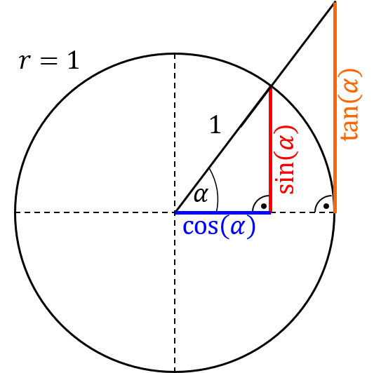
Um tan(α) am Einheitskreis zu visualisieren, konstruieren wir wieder ein rechtwinkliges Dreieck, bei dem dieses Mal die Ankathete zum Winkel α gleich eins ist. Die zugehörige Gegenkathete entspricht dann genau dem Tangens von α (siehe obere Abbildung).
Nach dem 2. Strahlensatz gilt:
tan(α)sin(α)=1cos(α)
Daraus folgt:
Variieren Sie in der folgenden Abbildung über den Schieberegler den Winkel α und beobachten Sie, wie sich die Werte für tan(α) ändern.
Da tan(α) für α=90°, α=270° bzw. α=−90° jeweils eine Polstelle besitzt, ist der einstellbare Winkelbereich entsprechend eingeschränkt.
import numpy as np
from bokeh.plotting import figure, show
from bokeh.models import Slider, ColumnDataSource, CustomJS, Label
from bokeh.layouts import column
from bokeh.io import output_notebook

output_notebook()

theta = np.linspace(0, 2*np.pi, 100)
x_circle = np.cos(theta)
y_circle = np.sin(theta)
alpha_init = 50
phi_init = np.deg2rad(alpha_init)

# Grunddaten für Startwinkel
tan_phi = np.tan(phi_init)
cos_phi = np.cos(phi_init)
sin_phi = np.sin(phi_init)

source_line = ColumnDataSource(data=dict(
    x0=[0, 1], y0=[0, 0],            # x-Achse
    x1=[0, 1], y1=[0, tan_phi],      # Tangens-Linie
    x2=[np.cos(phi_init), np.cos(phi_init)], y2=[0, sin_phi], # Sinus-Linie
    x3=[0, cos_phi], y3=[0, 0],      # Cosinus-Linie
    x4=[1, 1], y4=[0, tan_phi],      # Tangens-Linie vertikal
))

source_labels = ColumnDataSource(data=dict(
    x=[0.2, cos_phi, cos_phi/2, 1.1],
    y=[0.05, sin_phi/2, -0.15, tan_phi/2],
    text=[
        f"α={alpha_init}°",
        "sin(α)",
        "cos(α)",
        "tan(α)"
    ],
    color=["black", "red", "blue", "#FFA500"]
))

# Plot
p = figure(width=380, height=500, title="Einheitskreis", x_range=(-1.1, 1.1), y_range=(-1.1, 2.1))
p.line(x_circle, y_circle, line_color="gray", line_width=3)
p.line('x0', 'y0', source=source_line, line_color="black", line_dash="dashed")
p.line('x1', 'y1', source=source_line, line_color="black")
p.line('x2', 'y2', source=source_line, line_color="red", line_width=2)
p.line('x3', 'y3', source=source_line, line_color="blue", line_width=2)
p.line('x4', 'y4', source=source_line, line_color="#FFA500", line_width=2)
p.xaxis.axis_label = "x"
p.yaxis.axis_label = "y"
p.grid.grid_line_dash = [6, 4]

labels = LabelSet(
    x='x', y='y', text='text', text_color='color',
    text_font_size="12pt", source=source_labels,
    x_offset=0, y_offset=0
)
p.add_layout(labels)

# Slider für α (nur Werte, wo tan noch im Plot bleibt)
slider = Slider(start=0, end=85, value=alpha_init, step=1, title="α in °")

callback = CustomJS(args=dict(
    source_line=source_line,
    source_labels=source_labels,
    slider=slider
), code="""
    var alpha = slider.value;
    var phi = alpha * Math.PI / 180;
    var tan_phi = Math.tan(phi);
    var cos_phi = Math.cos(phi);
    var sin_phi = Math.sin(phi);

    // Linien aktualisieren
    source_line.data['x0'] = [0, 1];
    source_line.data['y0'] = [0, 0];
    source_line.data['x1'] = [0, 1];
    source_line.data['y1'] = [0, tan_phi];
    source_line.data['x2'] = [cos_phi, cos_phi];
    source_line.data['y2'] = [0, sin_phi];
    source_line.data['x3'] = [0, cos_phi];
    source_line.data['y3'] = [0, 0];
    source_line.data['x4'] = [1, 1];
    source_line.data['y4'] = [0, tan_phi];

    // Labels aktualisieren
    source_labels.data['x'] = [0.2, cos_phi, cos_phi/2, 0.8];
    source_labels.data['y'] = [0.05, sin_phi/2, -0.15, tan_phi/2];
    source_labels.data['text'] = [
        "α=" + alpha.toFixed(0) + "°",
        "sin(α)",
        "cos(α)",
        "tan(α)"
    ];
    source_labels.data['color'] = ["black", "red", "blue", "#FFA500"];

    source_line.change.emit();
    source_labels.change.emit();
""")

slider.js_on_change('value', callback)

layout = column(p, slider)
show(layout)Spezielle Werte der Winkelfunktionen
| Grad | 0° | 45° | 90° | 180° | 360° |
|---|---|---|---|---|---|
| Rad | 0 | 4π | 2π | π | 2π |
| sin(α) | 0 | 212 | 1 | 0 | 0 |
| cos(α) | 1 | 212 | 0 | -1 | 1 |
| tan(α) | 0 | 1 | Polstelle | 0 | 0 |